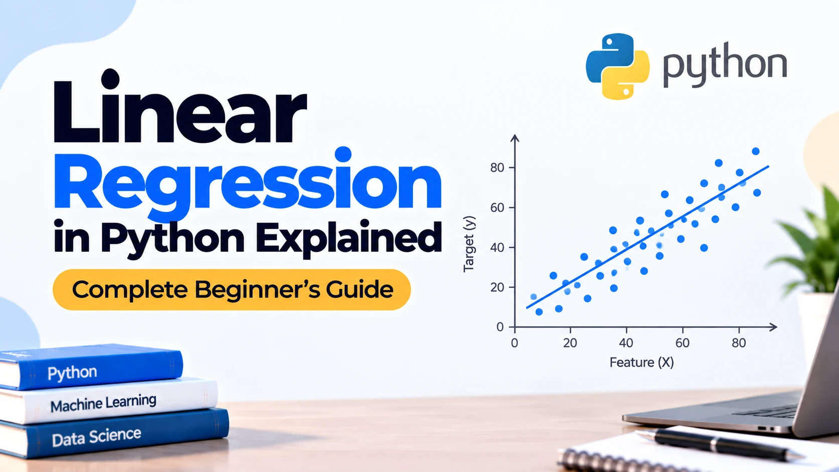
Linear Regression is one of the simplest and most important Machine Learning algorithms.

If you are learning Machine Learning with Python, Linear Regression is an excellent first algorithm because it introduces several fundamental concepts, including:

• Features and targets
• Training a model
• Making predictions
• Best-fit lines
• Model coefficients
• Model evaluation
• Training and test data
• Overfitting and underfitting

Linear Regression is mainly used when you want to predict a numerical value.

For example, you can use it to predict:

• House prices
• Salaries
• Sales
• Revenue
• Temperature
• Product demand
• Student scores
• Delivery time

Suppose you have this data:

Experience    Salary
1             30000
2             38000
3             45000
4             52000
5             60000

As experience increases, salary also appears to increase.

Linear Regression tries to learn this relationship and draw a line that best represents the data.

This guide explains Linear Regression in Python step by step using Pandas, Matplotlib, and scikit-learn.

What Is Linear Regression?

Linear Regression is a supervised Machine Learning algorithm used to model the relationship between one or more input variables and a numerical target.

For example:

Input:
Years of Experience

Output:
Salary

The algorithm tries to find a straight line that best represents the relationship between the variables.

For a simple Linear Regression problem, the relationship can be written as:

Predicted Value = Intercept + Coefficient × Input

It is commonly represented mathematically as:

ŷ = b₀ + b₁x

Where:

ŷ = Predicted value
b₀ = Intercept
b₁ = Coefficient or slope
x = Input feature

If the model learns:

Salary = 25000 + 7000 × Experience

then for someone with five years of experience:

Salary = 25000 + 7000 × 5

which gives:

60000

That is the basic idea behind Linear Regression.

Why Is It Called Linear Regression?

It is called linear because the model represents the relationship using a straight line.

Consider these points:

Experience    Salary
1             30000
2             37000
3             45000
4             51000
5             60000

When plotted, the points may approximately follow an upward straight-line pattern.

Linear Regression tries to find the line that fits these observations as closely as possible.

Regression vs Classification

Linear Regression solves a regression problem.

Regression predicts numerical values.

Examples:

House Price → 5,500,000

Salary → 65,000

Temperature → 31.5

Sales → 12,500

Classification predicts categories.

Examples:

Spam / Not Spam

Yes / No

Fraud / Not Fraud

Cat / Dog

So:

Numerical Output
→ Regression

Categorical Output
→ Classification

How Does Linear Regression Work?

Suppose we have:

Experience    Salary
1             30000
2             38000
3             45000
4             53000
5             60000

Linear Regression tries different possible lines and finds one that minimizes prediction errors.

Conceptually:

Actual Data Points
       ↓
Find Best-Fit Line
       ↓
Learn Relationship
       ↓
Predict New Values

The difference between an actual value and the model’s predicted value is called a residual or prediction error.

For example:

Actual Salary = 50000

Predicted Salary = 48000

Residual = 2000

The algorithm tries to find a line where these errors are collectively as small as possible.

What Is the Line of Best Fit?

The line of best fit is the straight line that best represents the relationship between the input and target values.

Imagine several data points:

Salary
  |
  |              *
  |          *
  |       *
  |    *
  | *
  |____________________
       Experience

Linear Regression places a line through the data approximately like:

Salary
  |
  |              * /
  |          *   /
  |       *    /
  |    *     /
  | *      /
  |____________________
       Experience

The line will usually not pass perfectly through every point.

Instead, it tries to minimize the overall errors.

What Is Least Squares?

A common method used by Linear Regression is called Ordinary Least Squares, or OLS.

The model calculates the difference between:

Actual Value

and:

Predicted Value

for every observation.

For example:

Actual       Predicted       Error
30000        31000           -1000
40000        39000            1000
50000        48000            2000

If we simply added the errors, positive and negative values could cancel each other.

Therefore, the errors are squared.

Conceptually:

Error²

The model then finds coefficients that minimize the sum of these squared errors.

This is why it is called least squares.

Simple Linear Regression vs Multiple Linear Regression

There are two common forms.

Simple Linear Regression

Simple Linear Regression uses one input feature.

Example:

Experience → Salary

The model looks like:

Salary =
Intercept +
Coefficient × Experience

Multiple Linear Regression

Multiple Linear Regression uses several input features.

For example:

Experience
Education
Age
Role Level
        ↓
      Salary

The model may look conceptually like:

Salary =
Intercept
+ b₁ × Experience
+ b₂ × Education
+ b₃ × Age

Both are Linear Regression models.

The difference is the number of input features.

Installing the Required Python Libraries

For this tutorial, install:

pip install pandas matplotlib scikit-learn

We will use:

import pandas as pd
import matplotlib.pyplot as plt

from sklearn.linear_model import LinearRegression

Create a Sample Dataset

Let’s create a simple dataset.

import pandas as pd

data = {
    "experience": [
        1,
        2,
        3,
        4,
        5,
        6,
        7,
        8,
        9,
        10
    ],
    "salary": [
        30000,
        36000,
        43000,
        51000,
        58000,
        65000,
        73000,
        81000,
        88000,
        96000
    ]
}

df = pd.DataFrame(data)

print(df)

Our dataset has:

Feature:
experience

Target:
salary

Step 1: Explore the Dataset

Before creating a model, inspect the data.

print(df.head())

Check its size:

print(df.shape)

Check data types:

print(df.dtypes)

Check missing values:

print(
    df.isnull().sum()
)

Generate statistics:

print(
    df.describe()
)

Even when working with a simple tutorial dataset, learning this habit is important.

Step 2: Visualize the Relationship

Create a scatter plot.

import matplotlib.pyplot as plt

plt.scatter(
    df["experience"],
    df["salary"]
)

plt.xlabel(
    "Years of Experience"
)

plt.ylabel(
    "Salary"
)

plt.title(
    "Experience vs Salary"
)

plt.show()

If the points roughly follow a straight-line pattern, Linear Regression may be a reasonable model to try.

Step 3: Define Features and Target

Create the feature variable:

X = df[
    ["experience"]
]

Create the target:

y = df[
    "salary"
]

Here:

X = Feature

y = Target

The uppercase X convention is commonly used because feature data is usually two-dimensional.

The lowercase y represents the target.

Step 4: Create the Linear Regression Model

Import:

from sklearn.linear_model import LinearRegression

Create the model:

model = LinearRegression()

At this point, the model has not learned anything.

Step 5: Train the Model

Use:

model.fit(
    X,
    y
)

The fit() method trains the model.

It learns the relationship between:

Experience

and:

Salary

After training, the model has learned:

• An intercept
• A coefficient

Step 6: Check the Coefficient

Use:

print(
    model.coef_
)

You may receive something similar to:

[7400]

This means the model estimates that salary increases by approximately 7,400 for each additional year of experience.

The exact number depends on your dataset.

Step 7: Check the Intercept

Use:

print(
    model.intercept_
)

You may receive something around:

21000

The learned relationship could therefore be approximately:

Salary =
21000 +
7400 × Experience

Step 8: Make Your First Prediction

Suppose someone has:

11 years of experience

Create the input:

new_data = pd.DataFrame({
    "experience": [
        11
    ]
})

Predict:

prediction = model.predict(
    new_data
)

print(
    prediction
)

The model returns an estimated salary.

You can access the first prediction:

print(
    prediction[0]
)

Complete Simple Linear Regression Example

Here is the complete program:

import pandas as pd
import matplotlib.pyplot as plt

from sklearn.linear_model import LinearRegression

data = {
    "experience": [
        1,
        2,
        3,
        4,
        5,
        6,
        7,
        8,
        9,
        10
    ],
    "salary": [
        30000,
        36000,
        43000,
        51000,
        58000,
        65000,
        73000,
        81000,
        88000,
        96000
    ]
}

df = pd.DataFrame(data)

X = df[
    ["experience"]
]

y = df[
    "salary"
]

model = LinearRegression()

model.fit(
    X,
    y
)

new_data = pd.DataFrame({
    "experience": [
        11
    ]
})

prediction = model.predict(
    new_data
)

print(
    "Coefficient:",
    model.coef_
)

print(
    "Intercept:",
    model.intercept_
)

print(
    "Predicted Salary:",
    prediction[0]
)

Visualize the Regression Line

We can visualize the line learned by the model.

First, predict all existing feature values:

predicted_salary = model.predict(
    X
)

Then plot:

plt.scatter(
    X["experience"],
    y,
    label="Actual Data"
)

plt.plot(
    X["experience"],
    predicted_salary,
    label="Regression Line"
)

plt.xlabel(
    "Years of Experience"
)

plt.ylabel(
    "Salary"
)

plt.title(
    "Linear Regression"
)

plt.legend()

plt.show()

The points represent actual observations.

The line represents predictions produced by the model.

Actual Value vs Predicted Value

Suppose:

Experience = 5
Actual Salary = 58000
Predicted Salary = 58200

The error is:

58000 - 58200 = -200

Some predictions will be above actual values.

Others may be below them.

A good regression line tries to minimize the overall errors.

Why We Should Use Train-Test Split

Our previous example trained the model using all available data.

That is useful for understanding Linear Regression, but it is not a good way to evaluate a real model.

We should separate the dataset into:

Training Data

and:

Test Data

Training data teaches the model.

Test data evaluates it on unseen examples.

Train-Test Split Example

Import:

from sklearn.model_selection import train_test_split

Split:

X_train, X_test, y_train, y_test = train_test_split(
    X,
    y,
    test_size=0.2,
    random_state=42
)

This means approximately:

80% → Training

20% → Testing

Train:

model = LinearRegression()

model.fit(
    X_train,
    y_train
)

Predict:

predictions = model.predict(
    X_test
)

Now we can properly evaluate the model.

Evaluate Linear Regression

Several metrics are commonly used to evaluate regression models.

Three important metrics are:

• Mean Absolute Error
• Mean Squared Error
• R-squared

Mean Absolute Error

Mean Absolute Error, or MAE, measures the average absolute difference between actual and predicted values.

Import:

from sklearn.metrics import mean_absolute_error

Calculate:

mae = mean_absolute_error(
    y_test,
    predictions
)

print(
    "MAE:",
    mae
)

Suppose:

MAE = 2500

This means the model’s predictions differ from actual values by about 2,500 on average for that test sample.

Lower MAE is generally better when comparing models on the same problem.

Mean Squared Error

Mean Squared Error, or MSE, squares prediction errors before calculating their average.

Import:

from sklearn.metrics import mean_squared_error

Use:

mse = mean_squared_error(
    y_test,
    predictions
)

print(
    "MSE:",
    mse
)

Because errors are squared, larger mistakes receive a stronger penalty.

Root Mean Squared Error

Root Mean Squared Error, or RMSE, is the square root of MSE.

Example:

import numpy as np

rmse = np.sqrt(
    mse
)

print(
    "RMSE:",
    rmse
)

RMSE is expressed in the same units as the target variable.

If the target is salary, RMSE is also expressed in salary units.

R-Squared

R-squared, also written as R², measures how well the model explains variation in the target compared with a simple baseline.

Import:

from sklearn.metrics import r2_score

Use:

r2 = r2_score(
    y_test,
    predictions
)

print(
    "R-squared:",
    r2
)

An R² value closer to 1 often indicates that the model explains more of the variation in the target.

However, R² should not be used alone to decide whether a model is good.

Always consider:

• The problem
• Test-set size
• Other metrics
• Residuals
• Business requirements

Complete Train-Test and Evaluation Example

import pandas as pd

from sklearn.model_selection import train_test_split
from sklearn.linear_model import LinearRegression
from sklearn.metrics import (
    mean_absolute_error,
    mean_squared_error,
    r2_score
)

data = {
    "experience": [
        1,
        2,
        3,
        4,
        5,
        6,
        7,
        8,
        9,
        10,
        11,
        12
    ],
    "salary": [
        30000,
        36000,
        43000,
        51000,
        58000,
        65000,
        73000,
        81000,
        88000,
        96000,
        102000,
        110000
    ]
}

df = pd.DataFrame(data)

X = df[
    ["experience"]
]

y = df[
    "salary"
]

X_train, X_test, y_train, y_test = train_test_split(
    X,
    y,
    test_size=0.25,
    random_state=42
)

model = LinearRegression()

model.fit(
    X_train,
    y_train
)

predictions = model.predict(
    X_test
)

mae = mean_absolute_error(
    y_test,
    predictions
)

mse = mean_squared_error(
    y_test,
    predictions
)

r2 = r2_score(
    y_test,
    predictions
)

print(
    "MAE:",
    mae
)

print(
    "MSE:",
    mse
)

print(
    "R-squared:",
    r2
)

Compare Actual and Predicted Values

Create a DataFrame:

results = pd.DataFrame({
    "Actual": y_test,
    "Predicted": predictions
})

print(results)

This is useful for manually inspecting prediction errors.

You can also calculate the errors:

results["Error"] = (
    results["Actual"]
    - results["Predicted"]
)

print(results)

What Are Residuals?

A residual is the difference between the actual value and predicted value.

Conceptually:

Residual =
Actual Value - Predicted Value

For example:

Actual = 70000

Predicted = 68000

Residual = 2000

Residual analysis can help determine whether Linear Regression is modeling the relationship appropriately.

Residual Plot

You can visualize residuals.

residuals = (
    y_test - predictions
)

plt.scatter(
    predictions,
    residuals
)

plt.axhline(
    y=0
)

plt.xlabel(
    "Predicted Values"
)

plt.ylabel(
    "Residuals"
)

plt.title(
    "Residual Plot"
)

plt.show()

Ideally, residuals should appear reasonably scattered around zero without an obvious systematic pattern.

Strong patterns may indicate that a straight-line model is not capturing the relationship well.

Multiple Linear Regression

Real-world predictions often depend on several variables.

Suppose salary depends on:

Experience
Age
Education Level

Create a dataset:

data = {
    "experience": [
        1,
        2,
        3,
        4,
        5,
        6,
        7,
        8
    ],
    "age": [
        22,
        24,
        26,
        29,
        31,
        34,
        36,
        40
    ],
    "education_years": [
        15,
        16,
        16,
        17,
        17,
        18,
        18,
        18
    ],
    "salary": [
        30000,
        38000,
        45000,
        55000,
        62000,
        72000,
        80000,
        92000
    ]
}

df = pd.DataFrame(data)

Define several features:

X = df[
    [
        "experience",
        "age",
        "education_years"
    ]
]

y = df[
    "salary"
]

Train:

model = LinearRegression()

model.fit(
    X,
    y
)

Now the model learns one coefficient for each feature.

Check them:

print(
    model.coef_
)

You can match them to feature names:

coefficients = pd.DataFrame({
    "Feature": X.columns,
    "Coefficient": model.coef_
})

print(coefficients)

Understanding Multiple Regression Coefficients

Suppose the model learns:

experience        6000
age                500
education_years   2000

The coefficient for experience represents the expected change in the predicted target associated with one additional unit of experience while the other included features remain fixed.

This is important.

In multiple regression, coefficients should not be interpreted without considering the other variables included in the model.

Linear Regression Assumptions

Linear Regression works best when several assumptions are reasonably satisfied.

1. Linear Relationship

The relationship between features and target should be approximately linear.

If the true relationship looks like:

Curved
Exponential
Highly irregular

a basic Linear Regression model may not capture it well.

2. Independent Observations

Observations should generally not improperly depend on one another.

For example, ordinary Linear Regression needs extra care when analyzing certain time-series or repeated-measures datasets.

3. Constant Error Variance

The spread of residuals should be reasonably consistent across prediction levels.

If residual variance grows dramatically as predictions increase, it may indicate heteroscedasticity.

4. Residual Normality

For some statistical inference uses of Linear Regression, approximately normally distributed residuals can matter.

For pure prediction, this assumption is often less central than whether the model generalizes well.

5. Limited Multicollinearity

In multiple Linear Regression, input features should not be excessively redundant with each other.

For example:

Age
Birth Year

may contain highly overlapping information depending on the dataset.

Strong multicollinearity can make coefficient interpretation unstable.

What Is Multicollinearity?

Multicollinearity happens when multiple input features are strongly related to one another.

Suppose:

Experience
Age

are extremely strongly correlated.

The model may struggle to determine how much influence should be assigned to each feature separately.

This can make coefficients unstable or difficult to interpret.

You can inspect correlations:

print(
    df.corr(
        numeric_only=True
    )
)

However, correlation alone does not fully diagnose every multicollinearity problem.

Does Linear Regression Require Feature Scaling?

Usually, standard Linear Regression does not require scaling just to produce predictions.

For example:

Age = 30

Salary-related feature = 80000

can still be handled.

However, scaling can be useful when:

• Comparing coefficient magnitudes
• Using regularized regression
• Combining preprocessing workflows
• Working with certain optimization-based models

So scaling is not always necessary for ordinary Linear Regression.

Linear Regression with a CSV File

Suppose you have:

salary_data.csv

containing:

experience,salary
1,30000
2,37000
3,45000
4,53000
5,60000

Load it:

import pandas as pd

df = pd.read_csv(
    "salary_data.csv"
)

Inspect:

print(
    df.head()
)

df.info()

print(
    df.isnull().sum()
)

Define data:

X = df[
    ["experience"]
]

y = df[
    "salary"
]

Then split and train normally.

What If the Dataset Has Missing Values?

Suppose:

experience    salary
1             30000
2             missing
3             45000

First investigate why the value is missing.

You might remove missing rows:

df = df.dropna(
    subset=[
        "experience",
        "salary"
    ]
)

For missing input features, imputation may be appropriate in some datasets.

Example:

from sklearn.impute import SimpleImputer

imputer = SimpleImputer(
    strategy="median"
)

The correct strategy depends on the problem.

Can Linear Regression Use Categorical Data?

Not directly as raw strings.

Suppose your dataset has:

City
Jaipur
Delhi
Mumbai

You generally need to encode the categories.

One common method is one-hot encoding.

Conceptually:

City_Jaipur
City_Delhi
City_Mumbai

Scikit-learn provides:

from sklearn.preprocessing import OneHotEncoder

For mixed numerical and categorical datasets, ColumnTransformer and pipelines are useful.

Linear Regression Pipeline Example

You can combine preprocessing and Linear Regression.

from sklearn.pipeline import Pipeline
from sklearn.impute import SimpleImputer
from sklearn.linear_model import LinearRegression

pipeline = Pipeline([
    (
        "imputer",
        SimpleImputer(
            strategy="median"
        )
    ),
    (
        "model",
        LinearRegression()
    )
])

Train:

pipeline.fit(
    X_train,
    y_train
)

Predict:

predictions = pipeline.predict(
    X_test
)

Pipelines help ensure preprocessing is applied consistently.

What Is Polynomial Regression?

Sometimes the relationship between variables is curved rather than straight.

For example:

y
|
|             *
|          *
|       *
|    *
| *
|________________ x

A straight line may not fit well.

Polynomial Regression creates additional features such as:

x
x²
x³

and then applies a linear model to those transformed features.

Scikit-learn provides:

from sklearn.preprocessing import PolynomialFeatures

However, increasing polynomial degree too much can cause overfitting.

Linear Regression vs Logistic Regression

These names sound similar, but they solve different problems.

Feature	Linear Regression	Logistic Regression
Problem	Regression	Classification
Output	Numerical value	Class probability/category
Example	House price	Spam detection
Example	Salary	Purchase Yes/No
Scikit-learn	LinearRegression	LogisticRegression

Do not use Linear Regression for a normal binary classification problem.

Linear Regression vs Decision Tree Regression

Linear Regression assumes an approximately linear relationship.

Decision Trees can model more complex nonlinear relationships.

Linear Regression is often:

• Easier to interpret
• Fast
• Simple
• Useful as a baseline

Decision Trees may capture:

• Nonlinear patterns
• Feature interactions
• Threshold-based relationships

Which performs better depends on the dataset.

Linear Regression vs Random Forest Regression

Random Forest combines many Decision Trees.

Compared with Linear Regression, it can model more complex relationships.

However, Random Forest is typically:

• More complex
• Harder to interpret
• More computationally demanding

Linear Regression remains valuable as a simple baseline.

What Is a Baseline Model?

A baseline model gives you a simple starting point for comparison.

For numerical prediction problems, Linear Regression can be an excellent baseline.

For example:

Linear Regression MAE = 5000

Random Forest MAE = 3500

The Random Forest may perform better on that dataset.

But without a baseline, it is harder to know whether the complex model actually provides meaningful improvement.

Overfitting in Linear Regression

Simple Linear Regression is less flexible than many complex models, but Linear Regression can still overfit, especially when:

• There are many features
• The dataset is small
• Polynomial terms are excessive
• Irrelevant features are included

For example:

Training Error = Very Low

Test Error = Much Higher

may indicate overfitting.

Underfitting in Linear Regression

Linear Regression may underfit when the real relationship is much more complex than a straight line.

For example:

Actual Relationship
→ Strong Curve

Model
→ Straight Line

The model may perform poorly on both training and test data.

Regularized Linear Regression

When datasets contain many features, you may encounter regularized versions of Linear Regression.

Two common examples are:

Ridge Regression

Lasso Regression

Ridge Regression

Ridge adds a penalty that discourages excessively large coefficients.

In scikit-learn:

from sklearn.linear_model import Ridge

Lasso Regression

Lasso can shrink some coefficients all the way to zero, depending on the data and regularization strength.

Import:

from sklearn.linear_model import Lasso

These techniques become useful when studying more advanced regression.

Practical House Price Example

Suppose we want to predict house prices from house size.

import pandas as pd

from sklearn.model_selection import train_test_split
from sklearn.linear_model import LinearRegression
from sklearn.metrics import mean_absolute_error

data = {
    "size": [
        800,
        1000,
        1200,
        1500,
        1800,
        2000,
        2200,
        2500,
        2800,
        3000
    ],
    "price": [
        2400000,
        3000000,
        3500000,
        4400000,
        5200000,
        5900000,
        6500000,
        7300000,
        8200000,
        9000000
    ]
}

df = pd.DataFrame(data)

X = df[
    ["size"]
]

y = df[
    "price"
]

X_train, X_test, y_train, y_test = train_test_split(
    X,
    y,
    test_size=0.2,
    random_state=42
)

model = LinearRegression()

model.fit(
    X_train,
    y_train
)

predictions = model.predict(
    X_test
)

mae = mean_absolute_error(
    y_test,
    predictions
)

print(
    "MAE:",
    mae
)

Predict the price of a 2,100-square-foot house:

new_house = pd.DataFrame({
    "size": [
        2100
    ]
})

price = model.predict(
    new_house
)

print(
    "Predicted Price:",
    price[0]
)

This is a simple example of how regression can be used for numerical predictions.

Practical Student Score Example

Suppose we want to predict exam scores from study hours.

data = {
    "study_hours": [
        1,
        2,
        3,
        4,
        5,
        6,
        7,
        8
    ],
    "score": [
        35,
        42,
        48,
        56,
        65,
        72,
        81,
        88
    ]
}

df = pd.DataFrame(data)

Define features:

X = df[
    ["study_hours"]
]

y = df[
    "score"
]

Train:

model = LinearRegression()

model.fit(
    X,
    y
)

Predict:

new_student = pd.DataFrame({
    "study_hours": [
        5.5
    ]
})

prediction = model.predict(
    new_student
)

print(
    prediction[0]
)

The model estimates the expected exam score based on the learned linear relationship.

When Should You Use Linear Regression?

Linear Regression can be a good choice when:

• Your target is numerical.
• The relationship is approximately linear.
• You want an interpretable baseline.
• You need fast training.
• Your dataset contains structured features.
• Understanding feature effects is important.

Examples include:

Salary Prediction

House Price Prediction

Revenue Prediction

Sales Forecasting

Demand Estimation

However, always verify whether the assumptions and predictive performance are reasonable for your specific data.

When Should You Avoid Linear Regression?

Linear Regression may not be the best option when:

• The target is categorical.
• Relationships are strongly nonlinear.
• Outliers severely distort the relationship.
• Important interactions are not represented.
• The data violates important assumptions.
• Another model performs significantly better on valid evaluation data.

Do not choose an algorithm only because it is easy.

Choose it based on the problem and evidence.

Advantages of Linear Regression

Easy to Understand

The relationship is represented using coefficients.

Fast to Train

Linear Regression is computationally efficient for many datasets.

Interpretable

Coefficients can often provide useful information about relationships between features and predictions.

Excellent Baseline

It provides a strong starting point before trying more complex models.

Works Well for Linear Relationships

When the underlying relationship is approximately linear, the model can perform very effectively.

Limitations of Linear Regression

Assumes a Linear Relationship

Complex nonlinear patterns may not be captured.

Sensitive to Outliers

Extreme values can influence the fitted line.

Multicollinearity Can Affect Interpretation

Highly correlated input features may make coefficients unstable.

Simple Model

Complex real-world relationships may require additional transformations or different algorithms.

Correlation Does Not Mean Causation

A Linear Regression coefficient represents an association within the model.

It does not automatically prove that changing one variable causes the target to change.

Common Mistakes to Avoid

1. Using Linear Regression for Classification

Do not use Linear Regression for:

Spam / Not Spam

Use a classification algorithm instead.

2. Training and Testing on the Same Data

Always create a proper test set when evaluating real model performance.

3. Ignoring Missing Values

Check:

df.isnull().sum()

before model training.

4. Ignoring Outliers

Extreme values can strongly influence a regression line.

Visualize your data before training.

5. Assuming Every Relationship Is Linear

Create scatter plots and inspect residuals.

Do not force Linear Regression onto clearly nonlinear data.

6. Using R-Squared Alone

Also consider:

MAE
MSE
RMSE
Residual Analysis

and the real-world meaning of errors.

7. Confusing Correlation with Causation

A strong coefficient or correlation does not prove cause and effect.

8. Adding Too Many Features

More features do not automatically create a better model.

Irrelevant features can add noise and make interpretation harder.

9. Ignoring Data Leakage

Preprocessing and feature selection should not improperly use information from the test set.

10. Making Predictions Far Outside the Training Range

Suppose your model was trained on:

Experience = 1 to 10 years

Predicting:

Experience = 50 years

requires extrapolation.

The learned linear relationship may not remain valid that far beyond the observed data.

Best Practices for Linear Regression

Start by understanding the business or research problem.

Plot the relationship between important variables.

Use:

df.describe()

to inspect distributions.

Check:

df.isnull().sum()

for missing values.

Investigate outliers.

Create a train-test split.

Train a simple baseline.

Evaluate using multiple relevant metrics.

Inspect residuals.

Compare Linear Regression with other reasonable models.

Keep preprocessing inside pipelines when the workflow becomes more complex.

Finally, interpret coefficients carefully and avoid making causal claims without supporting evidence.

Linear Regression Machine Learning Workflow

A practical workflow is:

Define Numerical Prediction Problem
             ↓
Collect Dataset
             ↓
Explore Data
             ↓
Clean Data
             ↓
Visualize Relationships
             ↓
Choose Features and Target
             ↓
Train-Test Split
             ↓
Train Linear Regression
             ↓
Make Predictions
             ↓
Evaluate MAE / MSE / R²
             ↓
Inspect Residuals
             ↓
Compare Other Models

How Linear Regression Connects to Becoming an AI Developer

Linear Regression is simple, but it teaches concepts used throughout Machine Learning.

You learn:

Features

Targets

Model Training

Predictions

Coefficients

Loss

Residuals

Train-Test Split

Evaluation

Generalization

These concepts continue appearing in:

Logistic Regression

Decision Trees

Random Forest

Neural Networks

Deep Learning

A strong AI learning path is:

Python
   ↓
NumPy
   ↓
Pandas
   ↓
Data Visualization
   ↓
EDA
   ↓
Statistics
   ↓
Scikit-Learn
   ↓
Linear Regression
   ↓
Logistic Regression
   ↓
Decision Trees
   ↓
Model Evaluation
   ↓
Feature Engineering
   ↓
Deep Learning

Understanding Linear Regression gives you a strong foundation for more advanced Machine Learning algorithms.

What to Learn Next

After Linear Regression, continue with:

1. Regression vs Classification
2. Logistic Regression
3. Mean Absolute Error
4. Mean Squared Error and RMSE
5. R-Squared Explained
6. Overfitting vs Underfitting
7. Cross-Validation
8. Polynomial Regression
9. Ridge Regression
10. Lasso Regression
11. Decision Tree Regression
12. Random Forest Regression
13. Feature Engineering
14. Hyperparameter Tuning
15. End-to-End Machine Learning Projects

A good progression is:

Linear Regression → Regression Metrics → Logistic Regression → Decision Trees → Random Forest → Model Evaluation → Advanced ML

Frequently Asked Questions

1. What is Linear Regression in Python?

Linear Regression is a supervised Machine Learning algorithm used to predict numerical values by learning an approximately linear relationship between input features and a target.

2. Which Python library is used for Linear Regression?

Scikit-learn provides the LinearRegression class:

from sklearn.linear_model import LinearRegression

3. What does model.fit() do?

model.fit() trains the Linear Regression model by learning coefficients and an intercept from the training data.

4. What does model.predict() do?

model.predict() uses the trained relationship to estimate target values for new feature data.

5. What is the difference between Linear Regression and Logistic Regression?

Linear Regression predicts numerical values, while Logistic Regression is primarily used for classification.

6. Does Linear Regression require feature scaling?

Ordinary Linear Regression does not usually require feature scaling just to make predictions, although scaling may be useful in some workflows and regularized models.

7. How do I evaluate a Linear Regression model?

Common evaluation metrics include Mean Absolute Error, Mean Squared Error, Root Mean Squared Error, and R-squared. Residual analysis is also useful.

8. Is Linear Regression good for beginners?

Yes. It is one of the best first Machine Learning algorithms because it teaches model training, prediction, coefficients, residuals, train-test splitting, and evaluation in an understandable way.

Conclusion

Linear Regression is one of the most fundamental algorithms in Machine Learning.

It learns an approximately linear relationship between input features and a numerical target, then uses that relationship to predict new values.

With Python and scikit-learn, you can build a Linear Regression model with only a few lines of code:

model = LinearRegression()

model.fit(
    X_train,
    y_train
)

predictions = model.predict(
    X_test
)

However, understanding the algorithm is more important than memorizing the code.

You should understand the role of coefficients, intercepts, residuals, train-test splitting, MAE, MSE, R-squared, assumptions, and data quality.

Linear Regression is also an excellent baseline for numerical prediction problems before moving to more complex algorithms.

Once you understand it well, the next logical topic is Logistic Regression in Python, where you move from predicting numbers to predicting categories.

---