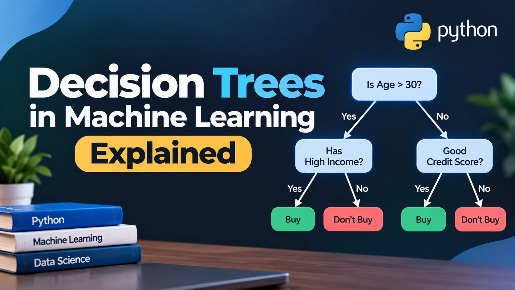
Decision Trees are one of the easiest Machine Learning algorithms to understand because they make predictions using a sequence of simple questions.

Instead of using a complex mathematical formula, a Decision Tree may behave like this:

Is income greater than 50,000?
        ↓
       Yes
        ↓
Is age greater than 30?
        ↓
       Yes
        ↓
Predict Purchase

This structure looks similar to a flowchart.

Decision Trees can be used for both:

• Classification
• Regression

For example, they can predict:

• Spam or Not Spam
• Customer Purchase or No Purchase
• Loan Approved or Rejected
• Customer Churn or Stay
• House Price
• Salary
• Sales
• Demand

In this guide, you will learn how Decision Trees work, important terms such as root nodes, branches, leaves, Gini impurity, entropy, tree depth, pruning, and how to build Decision Trees in Python using scikit-learn.

What Is a Decision Tree?

A Decision Tree is a supervised Machine Learning algorithm that makes predictions by splitting data into smaller groups based on feature values.

The structure resembles an upside-down tree.

A simple example:

               Income > 50,000?
                /           \
              No             Yes
             /                \
        No Purchase        Age > 30?
                           /       \
                         No         Yes
                    No Purchase   Purchase

Each question divides the dataset into groups.

The model continues splitting data until it reaches a prediction.

Why Is It Called a Decision Tree?

The algorithm has a tree-like structure made of:

• Root node
• Decision nodes
• Branches
• Leaf nodes

Conceptually:

Root Node
    ↓
Decision
   / \
  /   \
Branch Branch
 ↓       ↓
Leaf    Decision

The model starts from the root and follows branches until it reaches a leaf.

The leaf contains the final prediction.

Important Parts of a Decision Tree

Understanding the structure is essential.

Root Node

The root node is the first question in the tree.

For example:

Income > 50,000?

It represents the first and usually one of the most important splits.

Decision Node

A decision node asks another question.

For example:

Age > 30?

The answer determines which branch the data follows.

Branch

A branch connects nodes.

It represents the outcome of a question.

For example:

Yes

or:

No

Leaf Node

A leaf node is the final prediction.

For classification:

Purchase

or:

No Purchase

For regression:

Predicted Price = 5,500,000

How Does a Decision Tree Work?

Suppose you have customer data:

Age    Income    Purchased
22     25000     No
25     32000     No
30     45000     No
35     55000     Yes
40     70000     Yes
50     90000     Yes

The tree tries different ways to divide the data.

For example:

Income <= 45,000

may separate many non-buyers from buyers.

The algorithm evaluates possible splits and chooses one that creates groups that are as pure as possible.

Conceptually:

Mixed Data
    ↓
Choose Best Split
    ↓
Create Smaller Groups
    ↓
Repeat
    ↓
Final Predictions

What Is a Split?

A split divides observations based on a feature.

For example:

Age <= 30

creates:

Group 1:
Age <= 30

Group 2:
Age > 30

The algorithm searches for useful splits automatically.

For numerical features, it may test different thresholds.

For example:

Income <= 40,000

Income <= 50,000

Income <= 60,000

Then it chooses the split that best separates the target classes.

Decision Tree Classification

A Decision Tree classifier predicts categories.

Examples include:

Spam / Not Spam

Fraud / Not Fraud

Purchase / No Purchase

Pass / Fail

In scikit-learn, use:

from sklearn.tree import DecisionTreeClassifier

Decision Tree Regression

A Decision Tree regressor predicts numerical values.

Examples:

House Price

Salary

Revenue

Sales

Temperature

Use:

from sklearn.tree import DecisionTreeRegressor

Classification vs Regression Trees

Feature	Classification Tree	Regression Tree
Output	Category	Number
Example	Spam / Not Spam	House Price
Scikit-Learn	DecisionTreeClassifier	DecisionTreeRegressor
Split Goal	Separate classes	Reduce prediction error

Installing Required Libraries

Install:

pip install pandas scikit-learn matplotlib

Import:

import pandas as pd
import matplotlib.pyplot as plt

from sklearn.tree import DecisionTreeClassifier

Build a Simple Decision Tree Classifier

Let’s create a small customer-purchase dataset.

import pandas as pd

data = {
    "age": [
        20,
        22,
        25,
        28,
        30,
        35,
        38,
        42,
        45,
        50,
        55,
        60
    ],
    "income": [
        20000,
        24000,
        30000,
        35000,
        40000,
        50000,
        58000,
        65000,
        72000,
        85000,
        95000,
        110000
    ],
    "purchased": [
        0,
        0,
        0,
        0,
        0,
        1,
        1,
        1,
        1,
        1,
        1,
        1
    ]
}

df = pd.DataFrame(data)

print(df)

Here:

Features:
age
income

Target:
purchased

Step 1: Explore the Dataset

Check the first rows:

print(
    df.head()
)

Check shape:

print(
    df.shape
)

Check missing values:

print(
    df.isnull().sum()
)

Check class balance:

print(
    df["purchased"].value_counts()
)

Step 2: Define Features and Target

Create features:

X = df[
    [
        "age",
        "income"
    ]
]

Create target:

y = df[
    "purchased"
]

Step 3: Split Training and Test Data

Import:

from sklearn.model_selection import train_test_split

Split:

X_train, X_test, y_train, y_test = train_test_split(
    X,
    y,
    test_size=0.25,
    random_state=42,
    stratify=y
)

Now:

Training Data
→ Used to build the tree

Test Data
→ Used to evaluate it

Step 4: Create the Decision Tree Model

Create:

from sklearn.tree import DecisionTreeClassifier

model = DecisionTreeClassifier(
    random_state=42
)

Step 5: Train the Model

Use:

model.fit(
    X_train,
    y_train
)

The tree now learns useful decision rules from the training data.

Step 6: Make Predictions

Predict:

predictions = model.predict(
    X_test
)

print(
    predictions
)

The output may contain:

0
1

where:

0 = No Purchase

1 = Purchase

Step 7: Evaluate Accuracy

Import:

from sklearn.metrics import accuracy_score

Calculate:

accuracy = accuracy_score(
    y_test,
    predictions
)

print(
    "Accuracy:",
    accuracy
)

However, accuracy should not be the only metric you use for every classification problem.

Step 8: View the Confusion Matrix

Import:

from sklearn.metrics import confusion_matrix

Use:

matrix = confusion_matrix(
    y_test,
    predictions
)

print(matrix)

A confusion matrix helps show:

True Negative
False Positive
False Negative
True Positive

Complete Decision Tree Classification Example

import pandas as pd

from sklearn.model_selection import train_test_split
from sklearn.tree import DecisionTreeClassifier
from sklearn.metrics import (
    accuracy_score,
    confusion_matrix,
    classification_report
)

data = {
    "age": [
        20,
        22,
        25,
        28,
        30,
        35,
        38,
        42,
        45,
        50,
        55,
        60
    ],
    "income": [
        20000,
        24000,
        30000,
        35000,
        40000,
        50000,
        58000,
        65000,
        72000,
        85000,
        95000,
        110000
    ],
    "purchased": [
        0,
        0,
        0,
        0,
        0,
        1,
        1,
        1,
        1,
        1,
        1,
        1
    ]
}

df = pd.DataFrame(data)

X = df[
    [
        "age",
        "income"
    ]
]

y = df[
    "purchased"
]

X_train, X_test, y_train, y_test = train_test_split(
    X,
    y,
    test_size=0.25,
    random_state=42,
    stratify=y
)

model = DecisionTreeClassifier(
    random_state=42
)

model.fit(
    X_train,
    y_train
)

predictions = model.predict(
    X_test
)

print(
    "Accuracy:",
    accuracy_score(
        y_test,
        predictions
    )
)

print(
    confusion_matrix(
        y_test,
        predictions
    )
)

print(
    classification_report(
        y_test,
        predictions
    )
)

Visualize the Decision Tree

One major advantage of Decision Trees is that they can be visualized.

Import:

from sklearn.tree import plot_tree

Then:

plt.figure(
    figsize=(12, 7)
)

plot_tree(
    model,
    feature_names=X.columns,
    class_names=[
        "No Purchase",
        "Purchase"
    ],
    filled=True
)

plt.show()

The visualized tree shows:

• Split conditions
• Number of samples
• Class distribution
• Final prediction

This makes Decision Trees easier to explain than many other Machine Learning models.

How to Read a Decision Tree

You may see a node that looks similar to:

income <= 45000
gini = 0.49
samples = 9
value = [4, 5]
class = Purchase

Let’s understand each part.

income <= 45000

This is the condition used to split the data.

gini

This measures how mixed the classes are.

samples

This tells you how many training examples reached the node.

value

For example:

[4, 5]

may mean:

4 examples of Class 0

5 examples of Class 1

class

This is the predicted class at that node.

What Is Gini Impurity?

Gini impurity measures how mixed the classes are inside a node.

Consider a node containing:

10 Purchase
0 No Purchase

This node is completely pure.

Its impurity is very low.

Now consider:

5 Purchase
5 No Purchase

This node is highly mixed.

Its impurity is higher.

The tree tries to create splits that reduce impurity.

Simple Gini Intuition

Imagine:

Node A:
10 Cats
0 Dogs

This is pure.

Now:

Node B:
5 Cats
5 Dogs

This is mixed.

A Decision Tree prefers splits that turn mixed groups into purer groups.

What Is Entropy?

Entropy is another measure used to evaluate how mixed a node is.

A pure node has low entropy.

A highly mixed node has higher entropy.

Scikit-learn can use entropy by setting:

model = DecisionTreeClassifier(
    criterion="entropy",
    random_state=42
)

The default criterion for many classification tree workflows is Gini impurity.

Both aim to find useful splits.

Gini vs Entropy

Both Gini impurity and entropy measure node impurity.

Conceptually:

Gini
→ How mixed are the classes?

Entropy
→ How uncertain is the class distribution?

In many practical problems, they may produce similar trees.

You should generally evaluate model performance rather than assuming one criterion is always better.

What Is Information Gain?

Information gain measures how much a split reduces uncertainty.

Conceptually:

Information Gain =
Parent Impurity
-
Child Impurity

A useful split creates child nodes that are purer than the parent node.

The tree searches for splits with strong impurity reduction.

How Does a Tree Choose the Best Feature?

Suppose your features are:

Age
Income
Visits

The algorithm may test many possible splits such as:

Age <= 30

Income <= 50000

Visits <= 5

It evaluates how much each split improves purity.

The best split becomes the next node.

This process repeats recursively.

What Is Tree Depth?

Tree depth represents how many levels the tree contains.

For example:

Depth 0:
Root

Depth 1:
First Children

Depth 2:
Next Splits

A shallow tree is simpler.

A deep tree can learn more complicated patterns.

However, a very deep tree may overfit.

What Is max_depth?

Scikit-learn provides:

max_depth

to limit tree depth.

Example:

model = DecisionTreeClassifier(
    max_depth=3,
    random_state=42
)

This prevents the tree from growing beyond three levels.

Limiting depth is one of the simplest ways to control overfitting.

What Is Overfitting in Decision Trees?

Decision Trees can easily become too complex.

Suppose a tree keeps splitting until nearly every training observation has its own rule.

It may achieve:

Training Accuracy = 100%

but:

Test Accuracy = 72%

This is a common sign of overfitting.

The model has memorized training details instead of learning general patterns.

Why Decision Trees Overfit Easily

Trees can keep creating increasingly specific rules.

For example:

Age <= 31.5
Income > 52,432
Visits <= 7
Account Age > 13
...

A very detailed tree may fit noise rather than useful patterns.

Controlling tree complexity is therefore important.

How to Prevent Overfitting

Important parameters include:

max_depth

min_samples_split

min_samples_leaf

max_leaf_nodes

ccp_alpha

Let’s understand them.

min_samples_split

This controls the minimum number of samples required to split a node.

Example:

model = DecisionTreeClassifier(
    min_samples_split=10,
    random_state=42
)

A node with fewer than 10 samples will not be split.

This can reduce unnecessary complexity.

min_samples_leaf

This controls the minimum number of observations allowed in each leaf.

Example:

model = DecisionTreeClassifier(
    min_samples_leaf=5,
    random_state=42
)

This prevents leaves from containing extremely few examples.

max_leaf_nodes

This limits the total number of leaf nodes.

Example:

model = DecisionTreeClassifier(
    max_leaf_nodes=10,
    random_state=42
)

This can keep the tree compact.

What Is Pruning?

Pruning means reducing unnecessary branches from a Decision Tree.

Think of a real tree.

You cut unnecessary branches to make the structure simpler.

Machine Learning pruning works similarly.

The goal is:

Complex Tree
     ↓
Remove Weak Branches
     ↓
Simpler Tree
     ↓
Better Generalization

Cost Complexity Pruning

Scikit-learn provides:

ccp_alpha

for cost-complexity pruning.

Example:

model = DecisionTreeClassifier(
    ccp_alpha=0.01,
    random_state=42
)

Higher ccp_alpha usually encourages a smaller tree.

The best value should be selected using validation or cross-validation.

Feature Importance

Decision Trees can estimate feature importance.

Use:

print(
    model.feature_importances_
)

Match them with feature names:

importance = pd.DataFrame({
    "Feature": X.columns,
    "Importance": model.feature_importances_
})

print(
    importance.sort_values(
        "Importance",
        ascending=False
    )
)

You may see something like:

Feature    Importance
income     0.75
age        0.25

This suggests income contributed more strongly to the tree’s splits.

However, feature importance should be interpreted carefully.

It does not automatically mean that a feature causes the target outcome.

Do Decision Trees Need Feature Scaling?

Usually, no.

This is an important difference compared with algorithms such as:

• KNN
• SVM
• Logistic Regression

Suppose:

Age = 35

Income = 70000

A Decision Tree does not calculate distances between these features.

It uses threshold rules such as:

Age <= 35

Income <= 60000

Therefore, standard scaling is generally unnecessary.

Do Decision Trees Need One-Hot Encoding?

Scikit-learn Decision Trees require numerical input.

So raw text categories such as:

Jaipur

Delhi

Mumbai

still need to be converted into numerical features.

One common method is one-hot encoding.

Example:

from sklearn.preprocessing import OneHotEncoder

For mixed datasets, use:

ColumnTransformer

with a pipeline.

Decision Tree Pipeline Example

Suppose numerical columns contain missing values.

You can create:

from sklearn.pipeline import Pipeline
from sklearn.impute import SimpleImputer
from sklearn.tree import DecisionTreeClassifier

pipeline = Pipeline([
    (
        "imputer",
        SimpleImputer(
            strategy="median"
        )
    ),
    (
        "model",
        DecisionTreeClassifier(
            max_depth=4,
            random_state=42
        )
    )
])

Train:

pipeline.fit(
    X_train,
    y_train
)

Predict:

predictions = pipeline.predict(
    X_test
)

Decision Tree Regression Example

Now let’s predict house prices.

Create:

import pandas as pd

data = {
    "size": [
        800,
        1000,
        1200,
        1500,
        1800,
        2000,
        2200,
        2500,
        2800,
        3000
    ],
    "price": [
        2400000,
        3000000,
        3500000,
        4400000,
        5200000,
        5900000,
        6500000,
        7300000,
        8200000,
        9000000
    ]
}

df = pd.DataFrame(data)

Define:

X = df[
    ["size"]
]

y = df[
    "price"
]

Split:

from sklearn.model_selection import train_test_split

X_train, X_test, y_train, y_test = train_test_split(
    X,
    y,
    test_size=0.2,
    random_state=42
)

Create the regressor:

from sklearn.tree import DecisionTreeRegressor

model = DecisionTreeRegressor(
    max_depth=3,
    random_state=42
)

Train:

model.fit(
    X_train,
    y_train
)

Predict:

predictions = model.predict(
    X_test
)

print(
    predictions
)

Evaluate Decision Tree Regression

Use regression metrics.

Mean Absolute Error

from sklearn.metrics import mean_absolute_error

mae = mean_absolute_error(
    y_test,
    predictions
)

print(
    "MAE:",
    mae
)

Mean Squared Error

from sklearn.metrics import mean_squared_error

mse = mean_squared_error(
    y_test,
    predictions
)

print(
    "MSE:",
    mse
)

R-Squared

from sklearn.metrics import r2_score

r2 = r2_score(
    y_test,
    predictions
)

print(
    "R-squared:",
    r2
)

How Regression Trees Make Predictions

Classification trees predict categories.

Regression trees predict numerical values.

A regression tree may create rules such as:

House Size <= 1500?
      /        \
    Yes         No
     ↓           ↓
Price 3.5M   Size <= 2300?
                  /    \
                Yes     No
                 ↓       ↓
              5.8M     8.2M

Each leaf predicts a numerical value based on training observations that reached that leaf.

Decision Tree vs Linear Regression

Linear Regression fits a linear relationship.

Decision Trees use conditional rules.

Comparison:

Feature	Linear Regression	Decision Tree
Relationship	Linear	Can be nonlinear
Interpretability	High	High for small trees
Scaling Needed	Usually no	Usually no
Handles Interactions	Limited unless added	Naturally
Outlier Sensitivity	Can be high	Different behavior
Overfitting Risk	Usually lower	Can be high

A Decision Tree can learn relationships that are difficult to represent with a straight line.

Decision Tree vs Logistic Regression

Logistic Regression learns a linear classification boundary.

Decision Trees create rule-based boundaries.

For example, Logistic Regression may learn:

0.5 × Age
+
0.0001 × Income
→ Probability

A Decision Tree may learn:

Income > 50,000?

Yes → Age > 30?

No → No Purchase

Logistic Regression can be easier to interpret mathematically.

Decision Trees can capture nonlinear relationships and interactions naturally.

Decision Tree vs Random Forest

A Decision Tree uses one tree.

A Random Forest uses many trees.

Conceptually:

Decision Tree:
One Tree
→ One Prediction

Random Forest:

Tree 1
Tree 2
Tree 3
Tree 4
...
   ↓
Combine Predictions
   ↓
Final Prediction

A single Decision Tree is easier to explain.

Random Forest often provides better generalization because it combines multiple trees.

Decision Tree vs KNN

KNN predicts based on nearby examples.

Decision Trees predict using learned rules.

KNN:

Find Nearest Neighbors
→ Vote

Decision Tree:

Follow Conditions
→ Reach Leaf

KNN often requires feature scaling.

Decision Trees usually do not.

Decision Tree vs SVM

Support Vector Machines search for an effective separating boundary.

Decision Trees repeatedly split the feature space.

SVMs can work very well in certain high-dimensional problems.

Decision Trees are generally easier to visualize and explain.

Cross-Validation for Decision Trees

A single test split may produce unstable results.

Use cross-validation.

from sklearn.model_selection import cross_val_score
from sklearn.tree import DecisionTreeClassifier

model = DecisionTreeClassifier(
    max_depth=3,
    random_state=42
)

scores = cross_val_score(
    model,
    X,
    y,
    cv=5
)

print(
    scores
)

print(
    scores.mean()
)

Cross-validation is useful when comparing different tree configurations.

Hyperparameter Tuning

Decision Trees have several important hyperparameters.

Examples:

criterion

max_depth

min_samples_split

min_samples_leaf

max_leaf_nodes

ccp_alpha

You can use GridSearchCV.

Example:

from sklearn.model_selection import GridSearchCV
from sklearn.tree import DecisionTreeClassifier

model = DecisionTreeClassifier(
    random_state=42
)

parameters = {
    "max_depth": [
        2,
        3,
        4,
        5,
        None
    ],
    "min_samples_split": [
        2,
        5,
        10
    ],
    "min_samples_leaf": [
        1,
        2,
        5
    ]
}

search = GridSearchCV(
    model,
    parameters,
    cv=5
)

search.fit(
    X_train,
    y_train
)

print(
    search.best_params_
)

This searches multiple combinations automatically.

What Is random_state?

Decision Tree training can involve random behavior in certain situations.

Using:

random_state=42

helps make experiments reproducible.

This means your results are easier to reproduce when running the same code again.

Advantages of Decision Trees

Easy to Understand

Decision Trees use simple rules.

Easy to Visualize

You can display the complete decision process.

Works for Classification and Regression

The same basic approach can solve both types of problems.

Handles Nonlinear Relationships

Trees do not require a straight-line relationship.

Learns Feature Interactions

The tree can naturally create different rules depending on combinations of features.

No Standard Feature Scaling Required

Threshold-based splits generally do not require standardization.

Useful Baseline

A Decision Tree is often a good baseline before trying ensemble methods.

Limitations of Decision Trees

Easily Overfits

An unrestricted tree can become extremely complex.

Can Be Unstable

Small changes in the training data may produce a different tree.

Greedy Splitting

The algorithm usually chooses the best split at the current step rather than searching every possible future tree.

Complex Trees Become Hard to Interpret

Small trees are easy to explain.

Very large trees are not.

May Generalize Worse Than Ensembles

Random Forest and boosting methods often improve on the weaknesses of individual trees.

Real-World Use Cases

Decision Trees can be used in many areas.

Customer Churn

Features:

Subscription Length
Usage
Support Complaints
Monthly Payment

Prediction:

Churn / Stay

Loan Classification

Features:

Income
Credit History
Debt
Employment

Prediction:

Approve / Reject

Any real lending model must also consider applicable laws, fairness, bias, and appropriate human oversight.

Fraud Detection

Features:

Transaction Amount
Location
Device
Time

Prediction:

Fraud / Not Fraud

House Price Prediction

Features:

Size
Bedrooms
Location
Age

Prediction:

Price

Customer Purchase Prediction

Features:

Age
Income
Website Visits
Previous Orders

Prediction:

Purchase / No Purchase

Common Mistakes to Avoid

1. Allowing the Tree to Grow Without Limits

An unrestricted tree can easily overfit.

Try controlling:

max_depth
min_samples_leaf
min_samples_split

2. Evaluating on Training Data Only

Do not judge performance using the same examples used for training.

Use test data or cross-validation.

3. Assuming the Deepest Tree Is Best

A deeper tree fits training data more closely but may perform worse on new data.

4. Using Accuracy Alone

For imbalanced classification, also examine:

Precision
Recall
F1 Score
Confusion Matrix

5. Ignoring Missing Values

Check:

df.isnull().sum()

before model training.

6. Scaling Data Unnecessarily

Standard scaling is normally not required for tree-based models.

Do not add unnecessary preprocessing without understanding why.

7. Ignoring Class Imbalance

Check:

df["target"].value_counts()

before training.

8. Treating Feature Importance as Causation

A high feature importance score does not prove that a variable causes the outcome.

9. Using One Train-Test Split for Every Decision

Use cross-validation when comparing tree settings.

10. Ignoring Business Meaning

A technically accurate split may not always make practical sense.

Always interpret the model in the context of the actual problem.

Best Practices for Decision Trees

Start with a simple tree.

Use a train-test split.

Set random_state for reproducibility.

Visualize the tree.

Compare training and test performance.

Limit tree depth when necessary.

Use cross-validation to choose hyperparameters.

Evaluate with appropriate metrics.

Use pipelines when preprocessing is required.

Compare the Decision Tree with simpler and stronger alternatives.

For classification, compare against models such as Logistic Regression and Random Forest.

For regression, compare against Linear Regression and Random Forest Regression.

Decision Tree Workflow

A practical workflow is:

Define Problem
      ↓
Load Data
      ↓
Explore Dataset
      ↓
Clean Data
      ↓
Select Features and Target
      ↓
Train-Test Split
      ↓
Train Simple Tree
      ↓
Evaluate
      ↓
Visualize Tree
      ↓
Check Overfitting
      ↓
Tune Tree Depth
      ↓
Cross-Validate
      ↓
Compare Other Models

How Decision Trees Connect to Becoming an AI Developer

Decision Trees teach several important Machine Learning concepts:

Feature Splitting

Decision Rules

Impurity

Information Gain

Overfitting

Hyperparameters

Feature Importance

Classification

Regression

They also prepare you for more advanced tree-based algorithms.

A useful learning path is:

Python
   ↓
NumPy
   ↓
Pandas
   ↓
EDA
   ↓
Statistics
   ↓
Scikit-Learn
   ↓
Linear Regression
   ↓
Logistic Regression
   ↓
Decision Trees
   ↓
Random Forest
   ↓
Gradient Boosting
   ↓
Model Evaluation
   ↓
Feature Engineering
   ↓
Deep Learning

Decision Trees are especially important because several powerful Machine Learning algorithms are built using collections of trees.

What to Learn Next

After Decision Trees, continue with:

1. Random Forest in Python Explained
2. Gini Impurity Explained
3. Entropy and Information Gain
4. Overfitting vs Underfitting
5. Decision Tree Pruning
6. Feature Importance
7. Random Forest vs Decision Tree
8. Gradient Boosting
9. XGBoost
10. Classification Metrics
11. Cross-Validation
12. Hyperparameter Tuning
13. K-Nearest Neighbors
14. Support Vector Machines
15. Machine Learning Pipelines

A strong progression is:

Logistic Regression → Decision Trees → Random Forest → Gradient Boosting → Model Evaluation → Advanced Machine Learning

Frequently Asked Questions

1. What is a Decision Tree in Machine Learning?

A Decision Tree is a supervised Machine Learning algorithm that makes predictions by repeatedly splitting data according to feature-based rules.

2. Can Decision Trees be used for both classification and regression?

Yes. DecisionTreeClassifier is used for categorical targets, while DecisionTreeRegressor predicts numerical values.

3. Do Decision Trees require feature scaling?

Usually no. Decision Trees use threshold-based splits rather than distance calculations, so standard scaling is generally unnecessary.

4. What is Gini impurity?

Gini impurity measures how mixed the classes are inside a node. A purer node has lower impurity.

5. What is max_depth?

max_depth limits how many levels a tree can grow. It is commonly used to reduce model complexity and overfitting.

6. Why do Decision Trees overfit?

Trees can continue creating increasingly specific rules that memorize training data. Limiting depth, increasing minimum samples, or pruning can reduce this problem.

7. What is the difference between a Decision Tree and Random Forest?

A Decision Tree uses one tree. A Random Forest combines predictions from many trees, usually producing a more stable model.

8. Is a Decision Tree good for beginners?

Yes. Decision Trees are among the easiest Machine Learning algorithms to understand because their decisions can be visualized as simple rules.

Conclusion

Decision Trees are powerful and beginner-friendly Machine Learning algorithms that make predictions using a sequence of feature-based decisions.

They can solve both classification and regression problems and can model nonlinear relationships without requiring standard feature scaling.

With scikit-learn, creating a Decision Tree requires only a few lines:

model = DecisionTreeClassifier(
    max_depth=3,
    random_state=42
)

model.fit(
    X_train,
    y_train
)

predictions = model.predict(
    X_test
)

However, the most important concept to understand is model complexity.

An unrestricted Decision Tree can easily memorize training data and overfit.

Parameters such as max_depth, min_samples_split, min_samples_leaf, and pruning techniques help create simpler trees that generalize better.

Once you understand Decision Trees, the next logical step is Random Forest, which combines many Decision Trees to create a more stable and powerful Machine Learning model.

---